6 Recurrent Neural Networks
6.1 Motivation: Limitations of Feed-Forward Networks
Feed-forward networks have a fundamental limitation: they treat every input as an independent event. They have no built-in mechanism to understand sequence or time, which is a critical feature of most economic and financial data.
Examples in Economics Where Sequence Matters:
- Time Series Forecasting: Predicting future GDP, inflation, or stock prices depends on their historical path.
- Textual Analysis: The meaning of a word in a financial news article or policy document depends on the words that came before it.
- Consumer Behavior: A person’s next purchase is often influenced by their previous purchases.
A common workaround is to manually create features from past data, such as including lagged values (\(y_{t-1}, y_{t-2}, \dots\)) as inputs to a standard FNN. However, this requires pre-selecting a fixed window of history (the lag length \(p\)) and cannot gracefully handle long-range or variable-length dependencies. We need an architecture designed specifically for sequences.
6.2 The Core Idea of RNNs: A State That Remembers
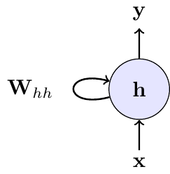
Recurrent Neural Networks (RNNs) solve this problem by introducing a loop. The network maintains a hidden state \(h\) (or “memory”), which captures information from all past steps. At each time step, the network updates this hidden state based on the current input and its previous state.
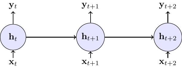
This can be visualized in two ways: a compact form with a self-loop, representing the recurrence, and an “unrolled” form, which shows the flow of information through time.
6.2.1 Mathematical Formulation
At each time step \(t\), the RNN performs the following calculations:
- \(\mathbf{x}_t \in \mathbb{R}^{D}\): The input vector at the current time step (e.g., today’s stock returns and trading volume).
- \(\mathbf{h}_{t-1} \in \mathbb{R}^{H}\): The hidden state from the previous time step, which acts as the network’s memory of the past.
- \(\mathbf{h}_t \in \mathbb{R}^{H}\): The new hidden state, calculated by combining the current input \(\mathbf{x}_t\) with the previous state \(\mathbf{h}_{t-1}\).
- \(\mathbf{y}_t \in \mathbb{R}^{O}\): The output at the current time step (e.g., the prediction for tomorrow’s volatility), produced from the current hidden state.
The update equations are:
\[ \begin{align} \mathbf{h}_t &= g(\mathbf{W}_{hh}\mathbf{h}_{t-1} + \mathbf{W}_{xh}\mathbf{x}_t + \mathbf{b}_h) \quad &\text{(Update memory)} \\ \mathbf{y}_t &= \mathbf{W}_{hy}\mathbf{h}_t + \mathbf{b}_y \quad &\text{(Produce output)} \end{align} \]
with the following parameters:
- \(\mathbf{W}_{hh} \in \mathbb{R}^{H \times H}\) (hidden-to-hidden weights)
- \(\mathbf{W}_{xh} \in \mathbb{R}^{H \times D}\) (input-to-hidden weights)
- \(\mathbf{W}_{hy} \in \mathbb{R}^{O \times H}\) (hidden-to-output weights)
- \(\mathbf{b}_h \in \mathbb{R}^{H}\), \(\mathbf{b}_y \in \mathbb{R}^{O}\) (bias terms)
In RNN implementations, the tanh function is often used as the activation function \(g\).
Key Properties:
- Parameter Sharing: The same weight matrices (\(\mathbf{W}_{hh}, \mathbf{W}_{xh}, \mathbf{W}_{hy}\)) and biases are used at every time step. This makes the model efficient and allows it to generalize across sequences of different lengths.
- Memory: The hidden state \(\mathbf{h}_t\) is the crucial component that allows information to persist, enabling the network to learn from context that appeared many steps in the past.
6.2.2 Econometric Intuition: RNN vs. GARCH Models
An RNN can be seen as a powerful, non-linear generalization of a classical time series model with hidden states like a GARCH model Bollerslev (1986).
In the GARCH(1,1) model, the latent conditional variance of stock returns is modeled as: \[ \sigma_t^2 = \omega + \alpha \varepsilon_{t-1}^2 + \beta \sigma_{t-1}^2 \]
Here, the “state” is the previous variance \(\sigma_{t-1}^2\), and the update rule is a simple linear function where \(\varepsilon_{t-1}\) is the demeaned return at time \(t-1\).
An RNN for the same task would be: \[ \begin{align} \mathbf{h}_t &= \tanh(\mathbf{W}_{hh}\mathbf{h}_{t-1} + \mathbf{W}_{xh}\mathbf{x}_t + \mathbf{b}_h) \\ \sigma_t^2 &= \text{softplus}(\mathbf{W}_{hy}\mathbf{h}_t + \mathbf{b}_y) \end{align} \]
Here, the hidden state \(\mathbf{h}_t\) is a high-dimensional vector that learns a much richer, non-linear summary of the entire relevant history contained in the input sequence \(\mathbf{x}_t\) (which could include past shocks \(\varepsilon_{t-1}^2\) and more). The RNN learns the optimal update function from data, rather than having it pre-specified as in GARCH.
The analogy with a GARCH model has its limits because a standard RNN produces a deterministic mapping \(y_t = f(h_t)\). By itself, this is not a probabilistic model. To align with the GARCH setup (which specifies a conditional distribution of returns), we need to wrap the RNN with a likelihood, e.g. for demeaned returns \(\varepsilon_t\):
- \(\varepsilon_t | h_t ∼ N(0, \sigma_t^2)\) with \(\sigma_t^2 = \text{softplus}(W_hy h_t + b_y)\), trained by (negative) log-likelihood.
- More generally, use natural gradient boosting or deep probabilistic layers to predict parameters of a chosen distribution.
6.2.3 Training: BPTT and the Vanishing Gradient Problem
Training an RNN presents a unique challenge due to its recurrent nature. Because the same weight matrices (\(\mathbf{W}_{hh}, \mathbf{W}_{xh}\)) are applied at every time step, their influence on the final loss is cumulative. The algorithm used to handle this is Backpropagation Through Time (BPTT).
The core idea of BPTT is to unroll the network through time, as shown in the diagram above. This conceptually transforms the RNN into a deep feed-forward network where each time step becomes a layer, but with the critical constraint that the weights are shared across all layers. Once unrolled, standard backpropagation can be applied.
The gradient for a weight matrix is the sum of its contributions at each time step. For example, the gradient with respect to \(\mathbf{W}_{hh}\) is: \[ \frac{\partial L_T}{\partial \mathbf{W}_{hh}}=\sum_{t=1}^{T}\frac{\partial L_T}{\partial \mathbf{h}_t}\frac{\partial \mathbf{h}_t}{\partial \mathbf{W}_{hh}} \]
The term \(\frac{\partial L_T}{\partial \mathbf{h}_t}\) captures how an adjustment to the hidden state at an early time \(t\) affects the final loss at time \(T\). This requires propagating the gradient backwards through every intermediate step, leading to a long product of Jacobian matrices: \[ \frac{\partial \mathbf{h}_t}{\partial \mathbf{h}_k} = \prod_{i=k+1}^{t} \frac{\partial \mathbf{h}_i}{\partial \mathbf{h}_{i-1}} = \prod_{i=k+1}^{t} \mathbf{W}_{hh}^{\top}\,\operatorname{diag}\big(g'(\mathbf{z}_i)\big) \]
where \(g'\) is the derivative of the activation function (e.g., \(\tanh'\)) and \(\mathbf{z}_i\) is its input at step \(i\). The detailed derivations for a one-dimensional hidden state can be found in a self-study exercise at the end of this section.
This long product is the source of the so-called vanishing gradient problem. If the norms of the weight matrix \(\mathbf{W}_{hh}\) and the activation derivatives are, on average, less than one, their repeated multiplication causes the gradient signal to shrink exponentially as it propagates back through time. Consequently, the contributions from early time steps (\(t \ll T\)) become so small that they are effectively zero. The network becomes unable to learn long-range dependencies, as its parameter updates are dominated by the most recent time steps.
If you ever implemented a GARCH model, you know that the likelihood depends on all past data and this makes estimation more complex.
The fundamental limitation of vanishing long-run dependence motivates the development of more advanced architectures like Long Short-Term Memory (LSTM) networks, which are designed to mitigate the vanishing gradient problem.
6.3 Exercises
In this exercise, we examine the vanishing gradient problem in RNNs. Consider a simple RNN with one-dimensional hidden state \(h_t = \tanh(W_h h_{t-1} + W_x x_t + b)\) and loss \(L_T\) at the final time step \(T\).
Tasks:
- Derive the gradient formula for backpropagation through time. Using the chain rule, derive the expression for \(\frac{\partial L_T}{\partial W_h}\). Show that it involves the term \(\frac{\partial h_T}{\partial h_t}\) for each time step \(t = 1, 2, \ldots, T\) and express it as a product of derivatives.
- Prove gradient vanishing conditions. Show that \(\left |\frac{\partial h_T}{\partial h_t}\right | \leq | W_h |^{T-t}\) and explain why this leads to exponentially vanishing gradients when \(|W_h | < 1\).
- Analyze learning implications. Explain why vanishing gradients prevent RNNs from learning long-term dependencies, including the effect on parameter updates for early time steps and typical sequence length limitations.
I extended the solution of part 1 with more explanations.
Technically at exam level. However, it’s hard to come up with variations of this exercise. Hence, any exam question would be very close to this setup.
For part 1, use the chain rule to express \(\frac{\partial L_T}{\partial W_h}\). Remember that the weight \(W_h\) affects the loss through its influence on all hidden states from time 1 to \(T\).
The key insight is that \(\frac{\partial L_T}{\partial W_h} = \sum_{t=1}^T \frac{\partial L_T}{\partial h_T} \frac{\partial h_T}{\partial h_t} \frac{\partial h_t}{\partial W_h}\).
For the product of derivatives, think about how \(h_T\) depends on \(h_t\) through the chain: \(h_t \to h_{t+1} \to h_{t+2} \to \cdots \to h_T\).
For part 2, you need to bound the absolute value of a product of derivatives. Use the property that \(|ab| = |a||b|\).
Each derivative \(\frac{\partial h_k}{\partial h_{k-1}}\) involves both the weight \(W_h\) and the derivative of the activation function. What’s the maximum value of \(\tanh'(z)\)?
For part 3, think about what happens to the gradient terms \(\frac{\partial L_T}{\partial W_h}\) when the \(\frac{\partial h_T}{\partial h_t}\) terms become very small for early time steps. How does this affect which time steps contribute most to parameter updates?
The goal is to find \(\frac{\partial L_T}{\partial W_h}\). The key challenge is that the weight \(W_h\) is used at every time step, so its influence on the final loss \(L_T\) is the sum of its influence through each step.
The final loss \(L_T\) is a function of the last hidden state, \(h_T\). But \(h_T\) is a function of \(h_{T-1}\) and \(W_h\). And \(h_{T-1}\) is a function of \(h_{T-2}\) and \(W_h\), and so on. This means that the final loss \(L_T\) is ultimately a function of \(W_h\) through its influence on every single hidden state:
\(L_T = f(h_T(h_{T-1}(...h_1(W_h)...), W_h), W_h)\)
Since \(W_h\) contributes to the final loss through all these paths, we have by the multivariate chain rule:
\[ \frac{\partial L_T}{\partial W_h} = \sum_{t=1}^T \frac{\partial L_T}{\partial h_t} \frac{\partial h_t}{\partial W_h} \]
Calculating the Direct Influence
The term \(\frac{\partial h_t}{\partial W_h}\) represents the direct influence of \(W_h\) on \(h_t\) at a single time step. From the RNN equation \(h_t = \tanh(W_h h_{t-1} + W_x x_t + b)\), this is straightforward: \[ \frac{\partial h_t}{\partial W_h} = \tanh'(W_h h_{t-1} + W_x x_t + b) \cdot h_{t-1} \]
Calculating the Indirect Influence (The Chain Rule Through Time)
The term \(\frac{\partial L_T}{\partial h_t}\) is more complex. It measures how a change in an early hidden state \(h_t\) propagates all the way to the end to affect the final loss \(L_T\). We must use the chain rule through the sequence of hidden states: \[ \frac{\partial L_T}{\partial h_t} = \frac{\partial L_T}{\partial h_T} \frac{\partial h_T}{\partial h_{T-1}} \frac{\partial h_{T-1}}{\partial h_{T-2}} \cdots \frac{\partial h_{t+1}}{\partial h_t} = \frac{\partial L_T}{\partial h_T} \prod_{k=t+1}^T \frac{\partial h_k}{\partial h_{k-1}} \] This long chain of derivatives is the core of backpropagation through time.
Now we can write the full expression for the gradient. Substituting our product form back into the sum at the beginning, we get \[ \frac{\partial L_T}{\partial W_h} = \sum_{t=1}^T \underbrace{\left( \frac{\partial L_T}{\partial h_T} \prod_{k=t+1}^T \frac{\partial h_k}{\partial h_{k-1}} \right)}_{\frac{\partial L_T}{\partial h_t}} \underbrace{\left( \frac{\partial h_t}{\partial W_h} \right)}_{\text{direct effect}} \] This formula explicitly shows that the gradient contribution from each time step \(t\) involves a product of terms that bridges the time gap from \(t\) to \(T\).
Each derivative in the product has the form: \[ \frac{\partial h_k}{\partial h_{k-1}} = \tanh'(W_h h_{k-1} + W_x x_k + b) \cdot W_h \]
Since \(\tanh'(z) = 1 - \tanh^2(z) \leq 1\), its value is always between 0 and 1. We can bound the absolute value of the derivative: \[ \left|\frac{\partial h_k}{\partial h_{k-1}}\right| = |\tanh'(\cdot)| \cdot |W_h| \leq 1 \cdot |W_h| = |W_h| \]
The key term \(\frac{\partial h_T}{\partial h_t}\) for \(t < T\) represents the product of derivatives through time: \[ \left|\frac{\partial h_T}{\partial h_t}\right| = \left|\prod_{k=t+1}^T \frac{\partial h_k}{\partial h_{k-1}}\right| \leq |W_h|^{T-t} \]
Exponential vanishing: When \(|W_h| < 1\), we have \(|W_h|^{T-t} \to 0\) exponentially as the time gap \((T-t)\) increases. This proves the exponential decay of gradient magnitudes.
The exponential decay has three critical effects on learning:
Dominated parameter updates: Since \(\frac{\partial L_T}{\partial W_h} = \sum_{t=1}^T \frac{\partial L_T}{\partial h_T} \frac{\partial h_T}{\partial h_t} \frac{\partial h_t}{\partial W_h}\), when \(\frac{\partial h_T}{\partial h_t}\) becomes exponentially small for early \(t\), the gradient sum becomes dominated by recent time steps (large \(t\)).
Loss of long-term information: The network cannot learn patterns where important information at time \(t\) influences the loss at time \(T\) when \(T-t\) is large, because the gradient signal carrying this information becomes negligibly small.
Practical sequence limitations: Empirically, standard RNNs can learn dependencies spanning roughly 5-10 time steps reliably. Beyond this, the exponential decay makes learning ineffective, limiting their applicability for sequences with long-term dependencies.
The fundamental issue is that learning requires non-negligible gradients to update parameters, but the exponential decay ensures that distant time steps contribute virtually nothing to parameter updates.
Consider a simple RNN with a single hidden unit processing a sequence of length 3. The RNN has the following parameters:
- Weight for input-to-hidden: \(W_{ih} = 0.5\)
- Weight for hidden-to-hidden: \(W_{hh} = 0.8\)
- Bias for hidden unit: \(b_h = 0.1\)
- Weight for hidden-to-output: \(W_{ho} = 1.2\)
- Bias for output: \(b_o = 0.0\)
The activation function for the hidden unit is \(\tanh\) and the output is linear (no activation). Given the input sequence \(\mathbf{x} = [0.2, -0.5, 0.3]\), compute the hidden states and outputs at each time step. Assume the initial hidden state \(h_0 = 0\).

Exam level difficulty
Work through each time step sequentially. Remember that the hidden state from the previous time step becomes input to the current time step. Use the fact that \(\tanh(0.2) \approx 0.197\), \(\tanh(0.008) \approx 0.008\), and \(\tanh(0.256) \approx 0.251\) to check your calculations.
The RNN equations are: \[ \begin{aligned} h_t &= \tanh(W_{ih} x_t + W_{hh} h_{t-1} + b_h) \\ y_t &= W_{ho} h_t + b_o \end{aligned} \]
Let’s compute step by step:
Time step 1 (\(t=1\)): \[ \begin{aligned} h_1 &= \tanh(0.5 \cdot 0.2 + 0.8 \cdot 0 + 0.1) \\ &= \tanh(0.1 + 0 + 0.1) \\ &= \tanh(0.2) \\ &\approx 0.197 \end{aligned} \] \[ \begin{aligned} y_1 &= 1.2 \cdot 0.197 + 0.0 \\ &\approx 0.236 \end{aligned} \]
Time step 2 (\(t=2\)): \[ \begin{aligned} h_2 &= \tanh(0.5 \cdot (-0.5) + 0.8 \cdot 0.197 + 0.1) \\ &= \tanh(-0.25 + 0.158 + 0.1) \\ &= \tanh(0.008) \\ &\approx 0.008 \end{aligned} \] \[ \begin{aligned} y_2 &= 1.2 \cdot 0.008 + 0.0 \\ &\approx 0.010 \end{aligned} \]
Time step 3 (\(t=3\)): \[ \begin{aligned} h_3 &= \tanh(0.5 \cdot 0.3 + 0.8 \cdot 0.008 + 0.1) \\ &= \tanh(0.15 + 0.006 + 0.1) \\ &= \tanh(0.256) \\ &\approx 0.251 \end{aligned} \] \[ \begin{aligned} y_3 &= 1.2 \cdot 0.251 + 0.0 \\ &\approx 0.301 \end{aligned} \]
Final Results: - Hidden states: \(h_1 \approx 0.197\), \(h_2 \approx 0.008\), \(h_3 \approx 0.251\) - Outputs: \(y_1 \approx 0.236\), \(y_2 \approx 0.010\), \(y_3 \approx 0.301\)