2 Cross Validation
2.1 How to Choose Hyperparameters and Architectures of Machine Learning Models?
When we build a machine learning model, we face several critical decisions that affect performance:
- Model Selection: Which algorithm should we use? (e.g., neural networks vs. random forests)
- Hyperparameter Tuning: What values should we choose for hyperparameters? (e.g., learning rate, regularization strength)
- Architecture Design: For neural networks, how many layers and neurons should we use?
Our primary goal is to create a model that performs well on new, unseen data. A model that only performs well on the data it was trained on is not useful in practice. This phenomenon, where a model learns the training data too well—including its noise and idiosyncrasies—is called overfitting.
2.2 The Problem with Simple Train-Test Splits
A simple approach is to split our data into a training set and a testing set:
- Train different models/configurations on the training set
- Evaluate their performance on the testing set
- Choose the best-performing option
However, this approach has major drawbacks:
- High variance: Model performance can be highly dependent on which specific data points ended up in each set
- Test set contamination: If we use the test set to make multiple decisions (choose hyperparameters, select architecture), we’re effectively “training” on the test set, leading to overly optimistic performance estimates
- Limited data usage: We’re not using all available data for training
Cross-validation provides a more robust and reliable method for both performance estimation and model selection by systematically using different subsets of the data for training and validation.
2.3 Cross-Validation for Model Selection
Cross-validation serves two main purposes:
Important
Two Key Uses of Cross-Validation
- Performance Estimation: Get a robust estimate of how well a model will perform on unseen data
- Model Selection: Choose between different hyperparameters, architectures, or algorithms based on their cross-validated performance
For neural networks specifically, cross-validation helps us choose:
- Number of hidden layers (network depth)
- Number of neurons per layer (network width)
- Learning rate and batch size
- Regularization parameters (dropout rate, weight decay)
- Activation functions and optimization algorithms
2.4 K-Fold Cross-Validation
The most common type of cross-validation is K-Fold Cross-Validation. The procedure is as follows:
- Shuffle the dataset randomly.
- Split the dataset into \(K\) equal-sized groups (or “folds”).
- For each fold:
- Use the fold as a validation set.
- Use the remaining \(K-1\) folds as a training set.
- Train the model on the training set and evaluate it on the validation set.
- Average the performance scores from the \(K\) folds to get a single, more robust performance estimate.
Common Choices for K
A common choice for \(K\) is 5 or 10. A higher \(K\) means less bias but can be computationally expensive. A lower \(K\) is faster but may have higher variance in its performance estimate.
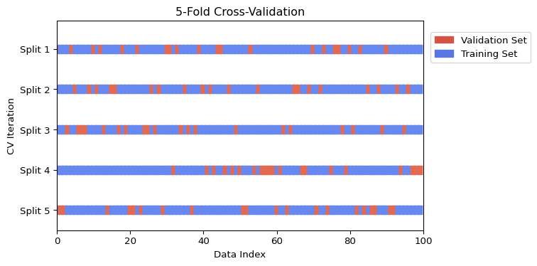
2.4.1 Visualizing K-Fold Cross-Validation
The following figure illustrates the K-Fold process for \(K=5\). In each iteration, a different fold is used for validation (orange) while the rest are used for training (blue).
Additional Information: Stratified K-Fold for Classification
When dealing with classification problems, especially with imbalanced classes, it’s typically important to use Stratified K-Fold. This variant ensures that each fold has the same percentage of samples for each class as the original dataset.
2.5 Time Series Cross-Validation
Standard K-Fold cross-validation is not suitable for time series data because it assumes that the data points are independent and identically distributed (i.i.d.). In time series, there is a temporal dependency; the order of the data matters. Randomly shuffling and splitting time series data would lead to data leakage, where the model is trained on data from the future to predict the past, leading to an overly optimistic performance estimate.
Specialized cross-validation techniques are needed for time series data.
2.5.1 Expanding Window (or Rolling-Origin)
In this approach, the training set grows with each split, and the validation set is always a block of data that comes after the training data.
- Start with a small training set.
- The next block of data is the validation set.
- In the next iteration, the previous validation set is added to the training set, and the subsequent block becomes the new validation set.
This mimics a real-world scenario where a model is periodically retrained as new data becomes available.
2.5.2 Sliding Window
This method uses a fixed-size training set that “slides” through time.
- Select a block of data for training.
- The next block of data is the validation set.
- In the next iteration, both the training and validation windows slide forward by a specified step.
This is useful when you believe that only the most recent data is relevant for prediction.
2.5.3 Visualizing Time Series Cross-Validation
The figure below illustrates the expanding and sliding window approaches.
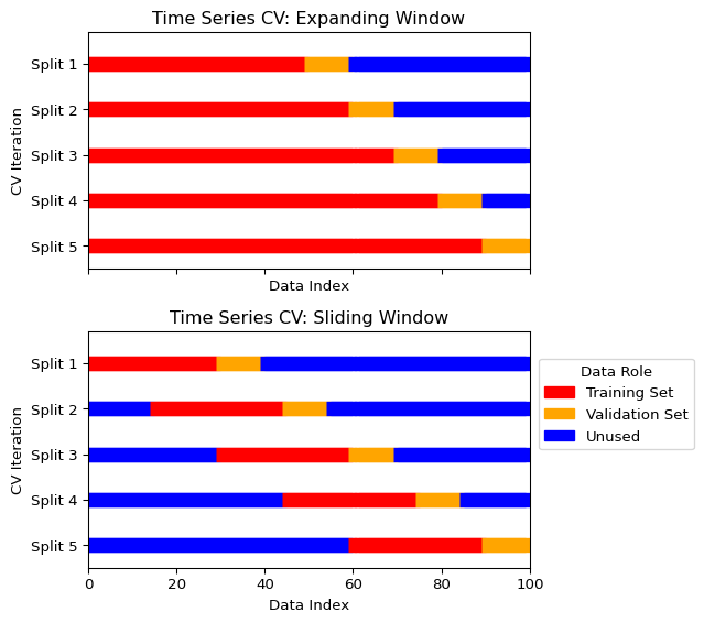
Scikit-learn’s TimeSeriesSplit implements the expanding window approach. A sliding window needs some self-coding.
2.6 Practical Example: Tuning a Neural Network with Cross-Validation
Let’s see how to use cross-validation to select the best hyperparameters for a simple neural network, see Section 5 . We’ll tune the number of hidden units and the learning rate using scikit-learn. Note that the sklearn implementation maximizes the negative mean squared error; that is, higher cross-validation score means better performance.
Show the code
import numpy as np
import matplotlib.pyplot as plt
from sklearn.neural_network import MLPRegressor
from sklearn.model_selection import cross_val_score, ParameterGrid
from sklearn.datasets import make_regression
from sklearn.preprocessing import StandardScaler
from sklearn.pipeline import Pipeline
import pandas as pd
import warnings

# Set random seeds for reproducibility
np.random.seed(42)

# Suppress convergence warnings
warnings.filterwarnings("ignore", category=UserWarning, module="sklearn")
warnings.filterwarnings("ignore", message="lbfgs failed to converge*")

# Generate synthetic dataset
X, y = make_regression(n_samples=1000, n_features=10, noise=0.1, random_state=42)

# Define hyperparameter grid
param_grid = {
    'hidden_layer_sizes': [(50,), (100,), (50, 50), (100, 50)],
    'learning_rate_init': [0.001, 0.01, 0.1],
    'alpha': [0.0001, 0.001, 0.01]  # L2 regularization
}

# Create pipeline with scaling
pipeline = Pipeline([
    ('scaler', StandardScaler()),
    ('mlp', MLPRegressor(max_iter=1000, random_state=42))
])

# Perform grid search with cross-validation
results = []
for params in ParameterGrid(param_grid):
    # Update pipeline parameters
    pipeline_params = {f'mlp__{key}': value for key, value in params.items()}
    pipeline.set_params(**pipeline_params)

    # Perform 5-fold cross-validation
    cv_scores = cross_val_score(pipeline, X, y, cv=5, scoring='neg_mean_squared_error')

    results.append({
        'hidden_layers': str(params['hidden_layer_sizes']),
        'learning_rate': params['learning_rate_init'],
        'alpha': params['alpha'],
        'mean_cv_score': cv_scores.mean(), # Convert to positive MSE
        'std_cv_score': cv_scores.std()
    })

# Convert to DataFrame for easier analysis
results_df = pd.DataFrame(results)

# Find best configuration
best_idx = results_df['mean_cv_score'].idxmax()
best_config = results_df.iloc[best_idx]

print("Best Configuration:")
print(f"Hidden Layers: {best_config['hidden_layers']}")
print(f"Learning Rate: {best_config['learning_rate']}")
print(f"Alpha (L2 reg): {best_config['alpha']}")
print(f"CV Score: {best_config['mean_cv_score']:.4f} ± {best_config['std_cv_score']:.4f}")

# Visualize results
fig, (ax1, ax2) = plt.subplots(1, 2, figsize=(12, 5))

# Plot 1: Learning rate vs performance (all configurations)
for alpha_val in results_df['alpha'].unique():
    subset = results_df[results_df['alpha'] == alpha_val]
    ax1.scatter(subset['learning_rate'], subset['mean_cv_score'],
               label=f'α={alpha_val}', alpha=0.7, s=50)

ax1.set_xlabel('Learning Rate')
ax1.set_ylabel('CV MSE')
ax1.set_title('Performance vs Learning Rate')
ax1.set_xscale('log')
ax1.grid(True, alpha=0.3)
ax1.legend(title='L2 Regularization')

# Plot 2: Architecture vs performance (all configurations)
# Create a mapping for architectures to x-positions
arch_names = results_df['hidden_layers'].unique()
arch_mapping = {arch: i for i, arch in enumerate(arch_names)}
results_df['arch_pos'] = results_df['hidden_layers'].map(arch_mapping)

# Add small random jitter to x-position for better visibility
np.random.seed(42)
jitter = np.random.normal(0, 0.05, len(results_df))

for lr_val in results_df['learning_rate'].unique():
    subset = results_df[results_df['learning_rate'] == lr_val]
    ax2.scatter(subset['arch_pos'] + jitter[subset.index], subset['mean_cv_score'],
               label=f'LR={lr_val}', alpha=0.7, s=50)

ax2.set_xlabel('Architecture')
ax2.set_ylabel('CV MSE')
ax2.set_title('Performance vs Architecture')
ax2.set_xticks(range(len(arch_names)))
ax2.set_xticklabels(arch_names, rotation=45)
ax2.grid(True, alpha=0.3)
ax2.legend(title='Learning Rate')

# Highlight best configuration
best_lr = best_config['learning_rate']
best_arch_pos = arch_mapping[best_config['hidden_layers']]
best_score = best_config['mean_cv_score']

ax1.scatter([best_lr], [best_score], color='red', s=100, marker='*',
           edgecolors='black', linewidth=1, label='Best Config', zorder=5)
ax2.scatter([best_arch_pos], [best_score], color='red', s=100, marker='*',
           edgecolors='black', linewidth=1, label='Best Config', zorder=5)

# Update legends to include best config
ax1.legend(title='L2 Regularization')
ax2.legend(title='Learning Rate')

plt.tight_layout()
plt.show()

# Show top 5 configurations
print("\nTop 5 Configurations:")
print(results_df.nlargest(5, 'mean_cv_score')[['hidden_layers', 'learning_rate', 'alpha', 'mean_cv_score', 'std_cv_score']])
Best Configuration:
Hidden Layers: (100,)
Learning Rate: 0.1
Alpha (L2 reg): 0.01
CV Score: -0.5821 ± 0.1241
Top 5 Configurations:
   hidden_layers  learning_rate   alpha  mean_cv_score  std_cv_score
29        (100,)            0.1  0.0100      -0.582092      0.124075
5         (100,)            0.1  0.0001      -0.584441      0.114173
17        (100,)            0.1  0.0010      -0.585387      0.113802
2          (50,)            0.1  0.0001      -0.621666      0.113096
26         (50,)            0.1  0.0100      -0.623375      0.122134
Key Insights from the Example
- Systematic Search: We test multiple combinations of hyperparameters systematically rather than guessing
- Robust Evaluation: Each configuration is evaluated using 5-fold cross-validation, giving us both mean performance and uncertainty estimates
- Fair Comparison: All models are evaluated on the same data splits, ensuring fair comparison
For Larger Networks
For deep neural networks with many hyperparameters, consider:
- Random Search: Sample hyperparameters randomly instead of exhaustive grid search
- Bayesian Optimization: Use libraries like
optunaorhyperoptfor more efficient search - Early Stopping: Monitor validation performance during training to avoid overfitting