9 Distributional Neural Networks
In many economic and financial applications, the signal-to-noise ratio is low, and decisions depend on the entire forecast distribution, not just a single point estimate. While standard deep learning models trained with Mean Squared Error (MSE) are powerful tools for estimating the conditional mean, \(\mathbb{E}[y|X]\), they often provide a poor and overconfident assessment of uncertainty.
Distributional Neural Networks address this by reframing the prediction problem. Instead of predicting a single value, the network predicts the parameters of a full probability distribution.
- Traditional NN Output: \(\hat{y} = f_\theta(\mathbf{x})\)
- Distributional NN Output: \(p(y|\mathbf{x}) = \text{Distribution}(\boldsymbol{\theta}(\mathbf{x}))\), where \(\boldsymbol{\theta}(\mathbf{x}) = f_\phi(\mathbf{x})\) are the distribution parameters learned by the network.
The model is trained by maximizing the log-likelihood of the data, which is equivalent to minimizing the negative log-likelihood loss: \[ \mathcal{L}(\phi) = -\sum_{i=1}^n \log p(y_i|\mathbf{x}_i; \boldsymbol{\theta}(\mathbf{x}_i)) \]
Of course, the optimization could also be done by another proper scoring rule like the continuous-ranked probability score.
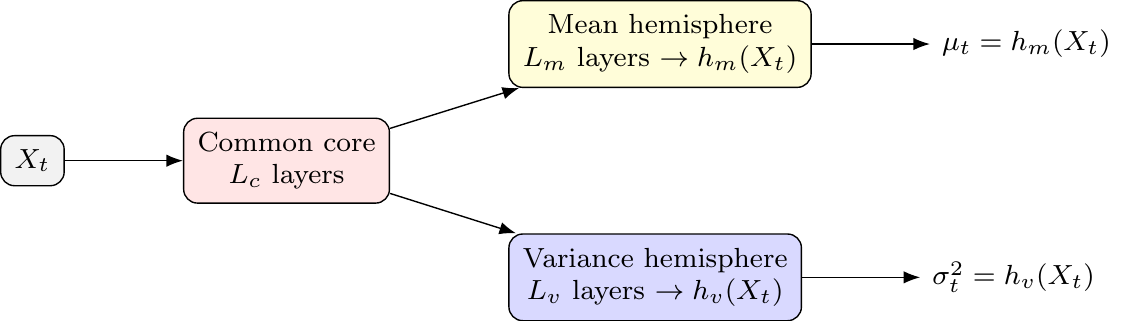
9.1 A Case Study: Hemisphere Neural Networks (HNN)
A key challenge in distributional modeling is reliably estimating multiple distribution parameters at once. Let’s consider the Gaussian case where we want to learn both the conditional mean and variance: \[ y_{t+1}\,|\,X_t \sim \mathcal{N}\big(\mu_t, \sigma_t^2\big),\quad \mu_t = f_\theta(x_t),\ \ \sigma_t^2 = g(x_t)>0 \] The per-time-step negative log-likelihood loss is (up to constants): \[ \ell_t(\theta,\phi)= \frac{(y_{t+1}-f_\theta(x_t))^2}{g(x_t)} + \log g(x_t) \] In highly overparameterized models, jointly training for \(\mu_t\) and \(\sigma_t^2\) via MLE is unstable. The model can achieve a low loss by either letting the mean network perfectly overfit (driving residuals and thus variance to zero) or by letting the variance network absorb all the variation. This is the “double descent” problem in a distributional context.
The Hemisphere Neural Network (HNN) architecture, proposed in a recent working paper by Goulet Coulombe, Frenette, and Klieber (2023), is designed to stabilize this process.
HNN Architecture
The core idea is to split the network after a shared “common core” into two specialized “hemispheres”—one for the mean and one for the variance.
- Common Core: A set of shared layers that learn a common representation. This allows latent drivers to influence both the mean and variance, creating an implicit link similar to ARCH or volatility-in-mean effects.
- Mean Hemisphere: A dedicated set of layers with a linear output head to predict \(\mu_t\).
- Variance Hemisphere: A dedicated set of layers with a
softplusoutput head to ensure the predicted variance \(\sigma_t^2\) is always positive.
This structure allows the model to learn both reactive volatility (where variance spikes after shocks, like in GARCH) and proactive volatility (where variance rises before shocks, based on leading indicators in \(x_t\)).
Stabilizing Joint MLE in Practice
The HNN framework introduces two key ingredients to discipline the unstable MLE procedure:
Volatility-Emphasis Constraint: Anchor the average predicted variance during training to a plausible level: \[ \frac{1}{T}\sum_t g(X_t) \approx \nu\cdot \operatorname{Var}(y) \] The target level \(\nu\) is determined from the out-of-bag residuals of a standard (non-distributional) neural network. This forces both hemispheres to contribute to the fit.
Blocked Subsampling (Time-Aware Bagging): The model is trained many times on different, non-overlapping time blocks (“bags”). The final predictions for \(\mu_t\) and \(\sigma_t^2\) are formed by averaging the predictions from models where time \(t\) was held out-of-bag. This stabilizes the predictions and makes them robust to initialization.
Practical Design Choices and Extensions
- Hyperparameters: A typical HNN might use 2 hidden layers for the core and 2 for each hemisphere, with ReLU activations, Adam optimization, and dropout.
- Beyond Gaussian: The hemisphere approach can be extended to other distributions (e.g., Student-t) by adding a third hemisphere for the degrees of freedom parameter, \(\nu\).
- Temporal Dynamics: To capture GARCH-like effects more directly, lagged outcomes or squared residuals can be included as features in \(X_t\). For more complex sequences, the common core could be an LSTM.
9.2 Handling Complex Distributions: Mixture Density Networks (MDNs)
For distributions that are skewed, fat-tailed, or multi-modal, a single parametric form is too restrictive. Mixture Density Networks (MDNs) proposed by Bishop (1994) address this by modeling the conditional distribution as a mixture of simpler ones, like Gaussians: \[ p(y|x)=\sum_{k=1}^K \pi_k(x)\,\mathcal{N}\!\big(y;\,\mu_k(x),\,\sigma_k^2(x)\big) \]
The network has three output heads to predict the parameters for all \(K\) components:
- Mixing Weights \(\pi_k(x)\): A
softmaxlayer ensures the weights are positive and sum to 1. - Means \(\mu_k(x)\): A linear layer.
- Standard Deviations \(\sigma_k(x)\): A
softpluslayer ensures positivity.
MDNs are particularly useful for modeling phenomena with distinct underlying states or regimes, which can lead to multi-modal distributions. Examples include:
- Multi-modal inflation distributions (e.g., a low-inflation vs. a high-inflation regime).
- Asset returns with regime switching behavior.
- Labor market dynamics that might feature multiple equilibria.
Unfortunately, MDNs can be challenging to train due to issues like component collapse (where one component dominates) and numerical instability from near-zero variances. These are often managed with careful initialization, regularization on mixing weights, and setting a minimum floor for \(\sigma_k\).
References
Bishop, Christopher. 1994. “Mixture Density Networks.” https://arxiv.org/abs/2012.03085.
Goulet Coulombe, Philippe, Mikael Frenette, and Karin Klieber. 2023. “From Reactive to Proactive Volatility Modeling with Hemisphere Neural Networks.” SSRN Electronic Journal. https://doi.org/10.2139/ssrn.4627773.