3 Evaluating Predictive Distributions

In many real-world applications, particularly in economics and finance, predicting a single value (a “point forecast”) is not enough. We often need to understand the full range of possible outcomes and their likelihoods. This requires us to move from point forecasts to distribution forecasts.

3.1 Distribution Forecasts vs. Point Forecasts

Let’s compare the two approaches:

• Point Forecasts:

  • Predict a single value, e.g., “tomorrow’s inflation will be 2.5%”.
  • This is often the conditional mean or median of the distribution.
  • Evaluated using metrics like Mean Squared Error (MSE) or Mean Absolute Error (MAE).

• Distribution Forecasts:

  • Predict an entire probability distribution for the future outcome, e.g., \(P(Y_{t+1} | \mathcal{F}_t)\).
  • Provides a complete picture of uncertainty, including variance, skewness, and tail risks.
  • More informative for decision-making, such as risk management or policy analysis.

Applications in Economics:

• Inflation Forecasting: Central banks are interested in the probability of inflation exceeding a certain target, not just the single most likely value.
• Risk Management: Financial institutions need to estimate the distribution of potential losses (e.g., Value-at-Risk at multiple risk levels).
• Policy Analysis: Governments need to understand the range of potential impacts of a new policy under uncertainty.

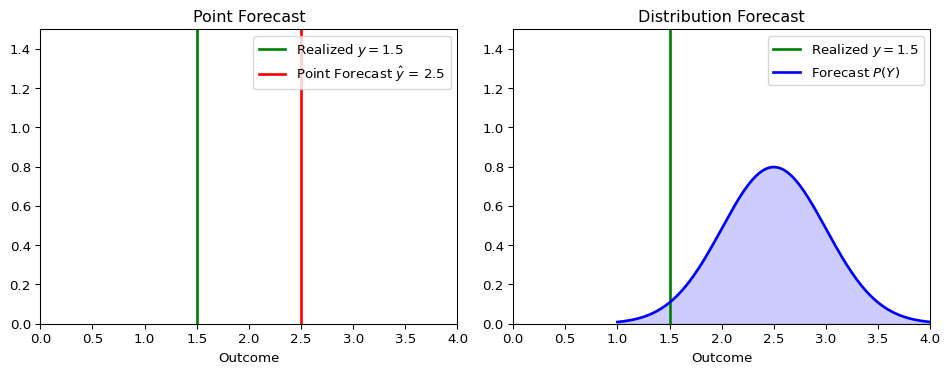
The figure below illustrates the conceptual difference.

Figure 1: Comparison of a point forecast and a distribution forecast.

A point forecast provides a single best guess, while a distribution forecast provides a richer view of what might happen.

3.2 Proper Scoring Rules

To evaluate a distribution forecast, we need a metric that assesses the quality of the entire predicted distribution, given the one outcome that actually occurred. This is the role of scoring rules.

A scoring rule \(S(P, y)\) assigns a numerical score to a forecast distribution \(P\) when the outcome \(y\) is realized, just like the MSE assign an error to a point forecast \(\hat y\) and \(y\).

Definition of Proper Scoring Rules

A scoring rule is considered proper if the forecaster’s expected score is optimized when they report their true belief (i.e., the true data-generating distribution). More precisely, let \(F\) and \(G\) be two distribution forecasts. A scoring rule \(S(P,y)\) that assigns a score to each combination of probability distribution \(P\) and outcome \(y\), is defined to be proper for some space of probability distributions \(\mathcal{P}\) if \[ \mathbb{E}_{Y \sim F}[S(F,Y)] \leq \mathbb{E}_{Y \sim F}[S(G,Y)] \]

for all \(F, G \in \mathcal{P}\). We call \(S\) strictly proper if the true distribution is the unique optimum.

This is analogous to how the conditional mean is the unique forecast that minimizes the Mean Squared Error. Using proper scoring rules incentivizes honest and accurate forecasting.

Optional: If you are interested in more technical details, see Gneiting and Raftery (2007).

Misunderstanding Proper Scoring Rules

• Proper doesn’t mean “better” - it means the rule encourages honest reporting
• Different proper scoring rules can rank models differently
• If possible, the choice of scoring rule should align with your specific decision problem

3.2.1 Why Proper Scoring Rules Matter

• They encourage forecasters to be honest and report their true beliefs.
• They provide a principled way to compare the performance of different forecasting models.
• They prevent “gaming” of evaluation metrics that might occur with simpler, ad-hoc measures, see below.

The Gaming Problem with Improper Scoring Rules

Suppose we evaluate forecasters using only the “hit rate” which we define to be zero when the realized outcome falls within their 90% prediction interval and 1 if the realization falls outside the prediction interval.

A Gaming Strategy: Given the hit rate evaluation, a strategic forecaster could report extremely wide intervals (e.g., [-1000, +1000] for inflation) to achieve a 100% hit rate while providing no useful information.

This would make the hit rate an improper scoring rule. Proper scoring rules include some sort of penalty to prevent such “underconfident” forecasts.

Two of the most widely used proper scoring rules are the Logarithmic Score (LogS) and the Continuous Ranked Probability Score (CRPS).

3.3 The Logarithmic Score (LogS)

The Logarithmic Score (or Log Score) evaluates the forecast density at the realized outcome.

Definition: For a forecast with probability density function (PDF) \(f\) and a realized outcome \(y\): \[\text{LogS}(f, y) = -\log f(y)\]

Properties:

• Lower scores are better.
• It is highly sensitive to tail events and severely penalizes a model that assigns a very low probability to an outcome that actually occurred.
• It requires an explicit forecast density \(f(y)\), which may not always be available.

Log Score: Visual Interpretation

The Log Score directly depends on the height of the density at the realized outcome \(y\). A forecas that assigns a higher probability to the value that actually occurs will receive a better (lower) score.

Figure 2: Visual interpretation of the Log Score. A higher density at the realized outcome y results in a better score.

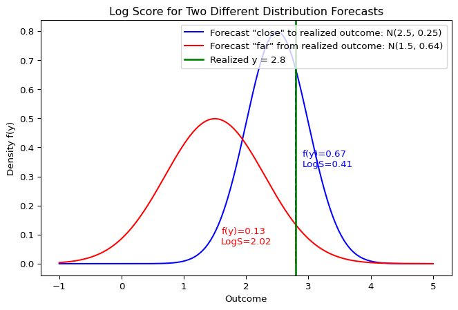
Example: Calculating the Log Score

Suppose we forecast that an outcome follows a Normal distribution \(Y \sim \mathcal{N}(\mu=2, \sigma^2=1)\), and the realized value is \(y = 2.5\).

import numpy as np
from scipy.stats import norm

mu, sigma = 2, 1
y_obs = 2.5

# Calculate the PDF value at the observed outcome
pdf_val = norm.pdf(y_obs, loc=mu, scale=sigma)
log_score = -np.log(pdf_val)

print(f"PDF value f({y_obs}) = {pdf_val:.4f}")
print(f"Log Score = {log_score:.4f}")

PDF value f(2.5) = 0.3521
Log Score = 1.0439

3.4 The Continuous Ranked Probability Score (CRPS)

The CRPS measures the “distance” between the forecast’s cumulative distribution function (CDF) and the empirical CDF of the outcome.

Definition: For a forecast with CDF \(F\) and a realized outcome \(y\): \[\text{CRPS}(F, y) = \int_{-\infty}^{\infty} [F(z) - \mathbf{1}\{z \geq y\}]^2 dz\] where \(\mathbf{1}\{z \geq y\}\) is the Heaviside step function, which represents the CDF of a perfect point forecast at \(y\).

Visual Interpretation

The CRPS measures the squared difference between the forecast CDF, \(F(z)\), and the empirical CDF of the outcome, which is a step function at \(y\). A steeply increasing CDF indicates that a lot of probability mass is concentrated in that region, leading to a smaller area if the outcome falls there. It can be visualized as the shaded area between these two curves.

Figure 3: Visual comparison of CRPS for a good (left) and a bad (right) forecast. The larger shaded area for the bad forecast corresponds to a higher (worse) CRPS score.

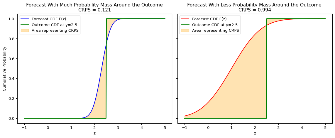
Intuition:

• It generalizes the Mean Absolute Error (MAE) to probabilistic forecasts. If the forecast is a single point, the CRPS reduces to the MAE. Even though it may not be intuitive at first sight given the square inside the integral, one can rewrite the CRPS as follows, \[ CRPS(F,y) = \mathbb{E} |X-y| - \frac{1}{2} \mathbb{E} |X-X'| \quad X,X'\stackrel{iid}{\sim}F. \]
• It considers both the location and the spread of the forecast distribution.
• It can be computed even if you only have samples from the forecast distribution, without needing an explicit density function.

Examples and Computation

For many standard distributions, the CRPS has a closed-form solution.

For a Normal Distribution: If the forecast is \(F = \mathcal{N}(\mu, \sigma^2)\), the CRPS is: \[\text{CRPS}(\mathcal{N}(\mu, \sigma^2), y) = \sigma\left[z\left(2\Phi(z) - 1\right) + 2\phi(z) - \frac{1}{\sqrt{\pi}}\right]\] where \(z = \frac{y - \mu}{\sigma}\), \(\Phi\) is the standard normal CDF, and \(\phi\) is the standard normal PDF.

More closed-form expressions can be found in Jordan, Krüger, and Lerch (2019).

Example: Calculating the CRPS

Using the same forecast \(Y \sim \mathcal{N}(\mu=2, \sigma^2=1)\) and outcome \(y = 2.5\) as above for the log score:

# Using the properscoring library for convenience
# pip install properscoring
import properscoring as ps

mu, sigma = 2, 1
y_obs = 2.5

crps_score = ps.crps_gaussian(y_obs, mu=mu, sig=sigma)
print(f"CRPS Score = {crps_score:.4f}")

CRPS Score = 0.3314

3.5 Comparing LogS vs. CRPS

Both are strictly proper scoring rules, but they have different sensitivities.

Aspect	Logarithmic Score (LogS)	Continuous Ranked Probability Score (CRPS)
Input Required	Forecast PDF, \(f(y)\)	Forecast CDF, \(F(y)\) (or samples)
Sensitivity	sensitive to tail performance; one bad miss can dominate the average score.	Less sensitive to outliers; focuses on the central tendency and overall shape.
Numerical Stability	Can be unstable if \(f(y)\) is close to zero.	Generally very stable.
Measurement Error Sensitivity	High	Low

3.6 Assessing Calibration with the Probability Integral Transform

I added this section on September 19

Beyond comparing models with scoring rules, we often want to diagnose how a model’s predictive distributions are failing. A powerful tool for this is the Probability Integral Transform (PIT).

The PIT is based on a fundamental statistical result: if a continuous random variable \(Y\) is drawn from a distribution with cumulative distribution function (CDF) \(F\), then the transformed random variable \(U = F(Y)\) follows a Uniform distribution on the interval [0, 1].

In forecasting, we can apply this principle to a sequence of forecasts and outcomes. If our model produces a series of predictive CDFs \(F_t\) for a series of outcomes \(y_t\), and if our forecasts are perfectly calibrated, then the resulting PIT values \(u_t = F_t(y_t)\) should be independent and identically distributed draws from a Uniform(0, 1) distribution.

We can visually check this by plotting a histogram of the PIT values. The shape of the histogram reveals systematic biases in the forecast distributions:

• Calibrated Forecasts: If the forecasts are well-calibrated, the PIT histogram will be approximately flat, resembling a uniform distribution.
• Underdispersed Forecasts (Too Narrow): If the forecast distributions are consistently too narrow, the realized outcomes will frequently fall in the tails. This leads to PIT values clustering near 0 and 1, creating a U-shaped histogram. The model is “overconfident” and surprised too often.
• Overdispersed Forecasts (Too Wide): If the forecast distributions are consistently too wide, the realized outcomes will tend to fall in the center of the distributions. This leads to PIT values clustering around 0.5, creating a hump-shaped histogram. The model is “underconfident” in its uncertainty.
• Miscalibrated Skewness: If the histogram is asymmetric or tilted, it indicates a mismatch in skewness. For example, an upward-sloping histogram (more values near 1) suggests the model’s forecasts are not sufficiently right-skewed compared to the outcomes. The model is systematically surprised by large positive outcomes.

import numpy as np
import matplotlib.pyplot as plt
from scipy.stats import norm, skewnorm

# --- Simulation Setup ---
n_samples = 5000
np.random.seed(42)

# --- Calculate PIT values for different forecast scenarios ---
# 1. Calibrated: True data is Normal, forecast is Normal
y_true_norm = norm.rvs(loc=0, scale=1, size=n_samples)
pit_calibrated = norm.cdf(y_true_norm, loc=0, scale=1)

# 2. Underdispersed: True data is Normal, forecast is too narrow
pit_underdispersed = norm.cdf(y_true_norm, loc=0, scale=0.5)

# 3. Overdispersed: True data is Normal, forecast is too wide
pit_overdispersed = norm.cdf(y_true_norm, loc=0, scale=2.0)

# 4. Skewness Mismatch: True data is skewed, forecast is symmetric Normal
skew_param = 5
y_true_skewed = skewnorm.rvs(a=skew_param, loc=0, scale=1, size=n_samples)
# Forecast with a Normal distribution matched to the true mean and std
mu_forecast = np.mean(y_true_skewed)
sigma_forecast = np.std(y_true_skewed)
pit_skew_mismatch = norm.cdf(y_true_skewed, loc=mu_forecast, scale=sigma_forecast)


# --- Plotting ---
fig, axes = plt.subplots(2, 2, figsize=(12, 8))
ax1, ax2, ax3, ax4 = axes.flatten()
bins = np.linspace(0, 1, 21)

# Calibrated
ax1.hist(pit_calibrated, bins=bins, density=True, color='skyblue', edgecolor='black')
ax1.axhline(1.0, color='red', linestyle='--', label='Uniform Density')
ax1.set_title('1. Calibrated Forecast')
ax1.set_ylabel('Density')
ax1.legend()

# Underdispersed
ax2.hist(pit_underdispersed, bins=bins, density=True, color='salmon', edgecolor='black')
ax2.axhline(1.0, color='red', linestyle='--')
ax2.set_title('2. Underdispersed (Too Narrow)')

# Overdispersed
ax3.hist(pit_overdispersed, bins=bins, density=True, color='lightgreen', edgecolor='black')
ax3.axhline(1.0, color='red', linestyle='--')
ax3.set_title('3. Overdispersed (Too Wide)')
ax3.set_xlabel('PIT Value')
ax3.set_ylabel('Density')

# Skew Mismatch
ax4.hist(pit_skew_mismatch, bins=bins, density=True, color='plum', edgecolor='black')
ax4.axhline(1.0, color='red', linestyle='--')
ax4.set_title('4. Miscalibrated Skewness')
ax4.set_xlabel('PIT Value')


for ax in axes.flatten():
    ax.set_ylim(0, max(ax.get_ylim()[1], 2.5)) # Ensure y-axis is comparable

plt.tight_layout()
plt.show()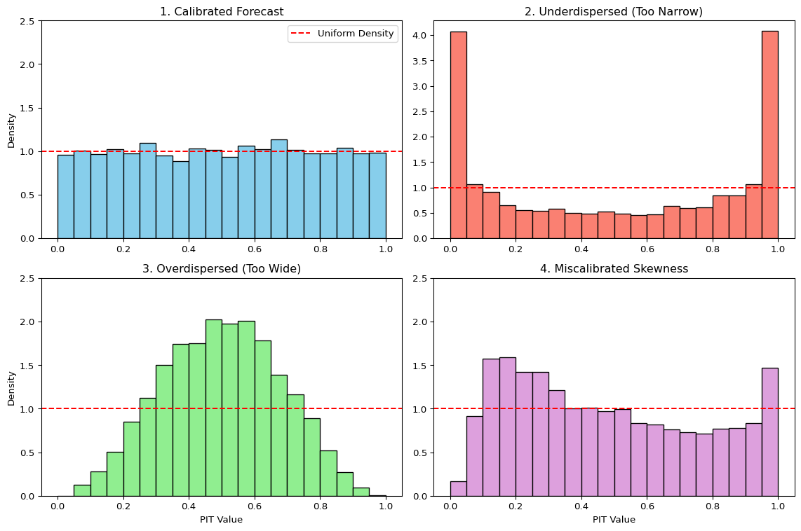

Figure 4: PIT histograms for calibrated, underdispersed, overdispersed, and skew-miscalibrated forecasts.

The PIT histogram is an powerful diagnostic tool. While a proper scoring rule gives a single number to rank models, the PIT histogram provides qualitative insights into why a model’s predictive distributions might be deficient, guiding further model improvement.

3.7 Deep dive: Connection to Information Theory

There is a deep connection between proper scoring rules and the concepts of entropy and cross-entropy discussed in the Information Theory chapter. This link is most direct for the Logarithmic Score.

Let’s assume there is a true, underlying data-generating distribution with density \(p(y)\), and our model produces a forecast distribution with density \(q(y)\).

The Log Score for a single observation \(y\) is: \[\text{LogS}(q, y) = -\log q(y)\]

To evaluate the quality of our forecasting model \(q\) in general, we consider its expected score under the true distribution \(p\):

\[ \mathbb{E}_{Y \sim p}[\text{LogS}(q, Y)] = \mathbb{E}_{Y \sim p}[-\log q(Y)] = -\int p(y) \log q(y) \,dy \]

This expression is exactly the definition of cross-entropy \(\mathbb{H}_{ce}(p, q)\) between the true distribution \(p\) and the forecast distribution \(q\).

3.7.1 Minimizing Log Score is Minimizing KL Divergence

Recall the fundamental relationship from information theory: \[ \underbrace{\mathbb{H}_{ce}(p, q)}_{\text{Expected Log Score}} = \underbrace{\mathbb{H}(p)}_{\text{Entropy of True Process}} + \underbrace{D_{\text{KL}}(p \parallel q)}_{\text{KL Divergence}} \]

This identity gives us a powerful interpretation:

1. Entropy \(\mathbb{H}(p)\): This is the irreducible uncertainty inherent in the true data-generating process. It represents the best possible average score we could ever achieve, even with a perfect model where \(q=p\).
2. KL Divergence \(D_{\text{KL}}(p \parallel q)\): This is the “penalty” or extra loss we incur because our model \(q\) is not a perfect representation of the true process \(p\). Since KL divergence is always non-negative (\(D_{\text{KL}} \geq 0\)), it represents the room for improvement in our model. This is very closely related to our argument in the section on Information Theory.

Key Insight

Minimizing the average Logarithmic Score of a forecast model is equivalent to minimizing the KL Divergence between the model’s predictive distribution (\(q\)) and the true data-generating distribution (\(p\)). This provides a theoretical foundation for using the Log Score in model selection and evaluation.

3.8 CRPS and Generalized Entropy

Last, we want to examine how the CRPS is also related to some form of “generalized entropy”. For a forecast CDF \(G\) and true CDF \(F\), the CRPS is \[\text{CRPS}(G,y)=\int_{-\infty}^{\infty}\big(G(z)-\mathbf{1}\{z \geq y\}\big)^2\,dz.\]

Taking expectation under \(Y \sim F\), \[ \begin{align} \mathbb{E}_{Y\sim F}[\text{CRPS}(G,Y)] &=\int \mathbb{E}\big[(G(z)-\mathbf{1}\{ z \geq Y\})^2\big]\,dz \\ &=\int (G(z)-F(z))^2\,dz+\underbrace{\int F(z)(1-F(z))\,dz}_{\mathbb H_{\text{CRPS}}(F)}, \end{align}\] where we used \(\mathbb E[\mathbf{1}(z \geq Y)]=F(z)\) and \(Var(\mathbf{1}(z \geq Y))=F(z)(1−F(z))\).

• The term \(\mathbb H_{CRPS}(F)=∫ F(1−F) dz\) is the generalized “CRPS entropy” of \(F\).
• The excess risk \[D_{\text{CRPS}}(F,G)=\int_{-\infty}^{\infty} (F(z)-G(z))^2\,dz\] is the Cramér–von Mises distance, showing CRPS is strictly proper (minimized at \(G(x)=F(x)\) for all \(x\)).

Equivalent representation: \[\mathbb H_{\text{CRPS}}(F)=\tfrac{1}{2}\,\mathbb{E}|X-X'|,\quad X,X'\stackrel{iid}{\sim}F,\] and \[\text{CRPS}(F,y)=\mathbb{E}|X-y|-\tfrac{1}{2}\mathbb{E}|X-X'| \quad X,X'\stackrel{iid}{\sim}F.\] The last expression can be used to define a multivariate CRPS analogue called “Energy Score”.

3.9 Key Takeaways

Essential Concepts for Distribution Forecasting

1. Distribution Forecasts Provide Richer Information

• Point forecasts give a single “best guess” but ignore uncertainty
• Distribution forecasts capture the full range of possible outcomes and their probabilities
• Critical for decision-making in economics, finance, and risk management

2. Proper Scoring Rules Enable Honest Evaluation

• Proper scoring rules incentivize forecasters to report their true beliefs
• They provide principled ways to compare different forecasting models

3. LogS vs. CRPS: Different Tools for Different Needs

• Logarithmic Score: Sensitive to tail events, requires explicit PDF
• CRPS: More robust to outliers, works with CDF or samples
• Both are strictly proper, but CRPS is generally more stable in practice

4. Connection to Information Theory

• Minimizing LogS is equivalent to minimizing KL divergence from the true distribution
• This provides theoretical foundation for why LogS works as an evaluation metric
• CRPS has analogous connections to generalized entropy measures

Beyond LogS and CRPS

• Energy Score for multivariate distributions (Székely and Rizzo 2005)
• Diebold-Mariano tests for comparing forecast performance (Diebold and Mariano 1995)
• Quantile scores for specific percentiles of interest (Gneiting and Raftery 2007)

References

Diebold, Francis X, and Robert S Mariano. 1995. “Comparing predictive accuracy.” Journal of Business and Economic Statistics 13 (3): 253–63. https://doi.org/10.1198.

Gneiting, Tilmann, and Adrian E. Raftery. 2007. “Strictly proper scoring rules, prediction, and estimation.” Journal of the American Statistical Association 102 (477): 359–78. https://doi.org/10.1198/016214506000001437.

Jordan, Alexander, Fabian Krüger, and Sebastian Lerch. 2019. “Evaluating probabilistic forecasts with scoringRules.” Journal of Statistical Software 90 (12): 1–37. https://doi.org/10.18637/jss.v090.i12.

Székely, Gábor J., and Maria L. Rizzo. 2005. “A new test for multivariate normality.” Journal of Multivariate Analysis 93 (1): 58–80. https://doi.org/10.1016/j.jmva.2003.12.002.